Gerschgorin Disks

Lately I’ve been reviewing my linear algebra and was reminded of an interesting result that we only briefly touched on in my first graduate linear algebra class: the Gerschgorin Disk Theorem. It’s interesting because it gives a straightforward way to bound the locations of the eigenvalues of a matrix in the complex plane in terms of its diagonal entries and row sums (not including diagonal entries). The diagonal entries determine the centers of the disks, while the radius is determined by difference in magnitude between the diagonal entry and its corresponding row sum (not including the diagonal). Perhaps I shouldn’t be surprised that what may seem like arbitrary quantities — row sums and diagonal entries — tell us quite a bit about the nature of matrix, but I still do.

Not finding a simple function to visualize these disks in Mathematica, I implemented my own:

GerschgorinPlot[A_] := 
 (* Store the number of rows in A *)
 With[{n = Dimensions[A][[1]]},
  Show[
   (* Plot the eigenvalues as points *)
   ListPlot[{Re[#], Im[#]} & /@ Eigenvalues[A], AxesOrigin -> {0, 0}, 
	AspectRatio -> Automatic, PlotRange -> All, 
	PlotStyle -> PointSize[Medium]],
   (* Create a translucent gray disk for each row *)
   {Graphics[{EdgeForm[Thin], GrayLevel[0.1, 0.1], 
	    Disk[{Re[#1], Im[#1]}, #2]}]} & @@@ Thread[{
	  (* Disk centers *)
	  Table[A[[i, i]], {i, 1, n}],
	  (* Disk radii *)
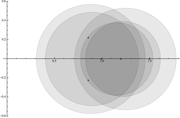
	  Table[Total[Abs[A[[i]]], i] - Abs[A[[i, i]]], {i, 1, n}]}]]]

It plots the eigenvalues as points in addition to the Gerschgorin disks. Here’s a sample of the output for a slightly perturbed 5th-order identity matrix:

I’m fairly pleased with the result, but will continue to tweak it. If you prefer MATLAB, you might have a look at this implementation.