Julia in Julia
For some time now, I’ve meant to write about Julia, a new programming language specifically designed for scientific computing. Julia is a young language — it’s been around for around two years now — that has a lot to offer. It’s a dynamic language like MATLAB or Python, but includes a sophisticated type system that stays out of the way (via type inference) when you don’t want it. Perhaps more interesting is Julia’s first-class support for multiple dispatch. The language and libraries are rooted in this paradigm, and it works well. On top of all that, Julia has excellent performance, that often compares favorably to C, let alone Python or MATLAB.
Julia’s name evokes images of the Julia set, a well-known fractal. For fun and visual interest, I chose to use Julia to generate some images of the Julia set. This has the additional benefit of allowing us to demonstrate the use of some popular Julia packages, such as those for working with image and color.
The fractals I’m going to be working with all result from considering the orbits of a function over a set of points in the complex plane. Now, in case you aren’t familiar with the concept, an orbit is the sequence of points generated from repeated application of a function to an initial seed point, i.e. \[ x_0, f(x_{0}), f(f(x_{0})), \ldots, f^n(x_{0}), \ldots \] The incredible structures that we see in well-known images of fractals like the Julia set or Mandelbrot set emerge from considering whether this sequence (orbit) is bounded, or escapes to infinity. To that end, we will require a function that, given a function and a seed, will determine whether the orbit is bounded, which leads to our first bit of Julia code:
function boundedorbit(f, seed, bound, iterations=100, itmap=(n,zn,b)->n)
    z = f(seed)
    for k = 1:iterations
        if abs(z) > bound
            return itmap(k, z, iterations)
        end
        z = f(z)
    end
    return -Inf
end
Now, of course we cannot guarantee that just because the first \(n\) terms of a given orbit are bounded, that the orbit will not eventually diverge, hence we impose a limit on the number of iterations after which we simply assume that the orbit is bounded. This limit is sometimes referred to as the bailout radius.
Let’s try this function on a particular seed value for the function \(z \mapsto z^2 - 1\):
boundedorbit(z -> z^2 - 1, 1, 2)-Inf
I love that the syntax for the anonymous function z -> z^2 - 1 is so similar to the mathematical notation. Notice that a different seed value results in an orbit that is not bounded:
boundedorbit(z -> z^2 - 1, 1 + 1im, 2)1
As you would expect, the seed value of \(1+1i\) exceeds the bound of \(2\) in just one step.
To generate an image, we’re going to need two more tools. First, a way to generate a (rectangular) set of points from the complex plane. We can then apply boundedorbit to each point in that set. Now Julia already includes a linspace function for generating equally spaced points between two endpoints; it’s a shame that out-of-the box there is no specialization of this function for the Complex type, generating an equally spaced grid of points between two numbers in the complex plane. No matter, Julia allows us to introduce just such a function:
import Base.linspace

function linspace(start::Complex, finish::Complex, n::Integer, m::Integer)
    realParts = linspace(real(start), real(finish), n)
    complexParts = [Complex(0, b) for b=linspace(imag(start), imag(finish), m)]
    [ a + b for a=realParts, b=complexParts ]
end
This illustrates just a tiny bit of the power of multimethods. Now we’re going to need a way to map the numbers generated by boundedorbit (the number of iterations required to escape) to color values. The simplest approach to begin with is to treat these numbers as grayscale values; in this case we map the iteration count into an 8-bit integer (0..255) so that the resulting data can be readily converted to a grayscale image.
function grayvalue(n)
    if n == -Inf
        Uint8(0)
    else
        Uint8(iround(clamp(n, typemin(Uint8), typemax(Uint8))))
    end
end
At this point we have just about enough to produce a decent image of the Julia set.
points = linspace(-2-1im, 2+1im, 2000, 1000));
values = map(z -> boundedorbit(x -> x^2 - 1, z, 2, 200)
               |> x -> 10x
               |> grayvalue, points);
image = grayim(values)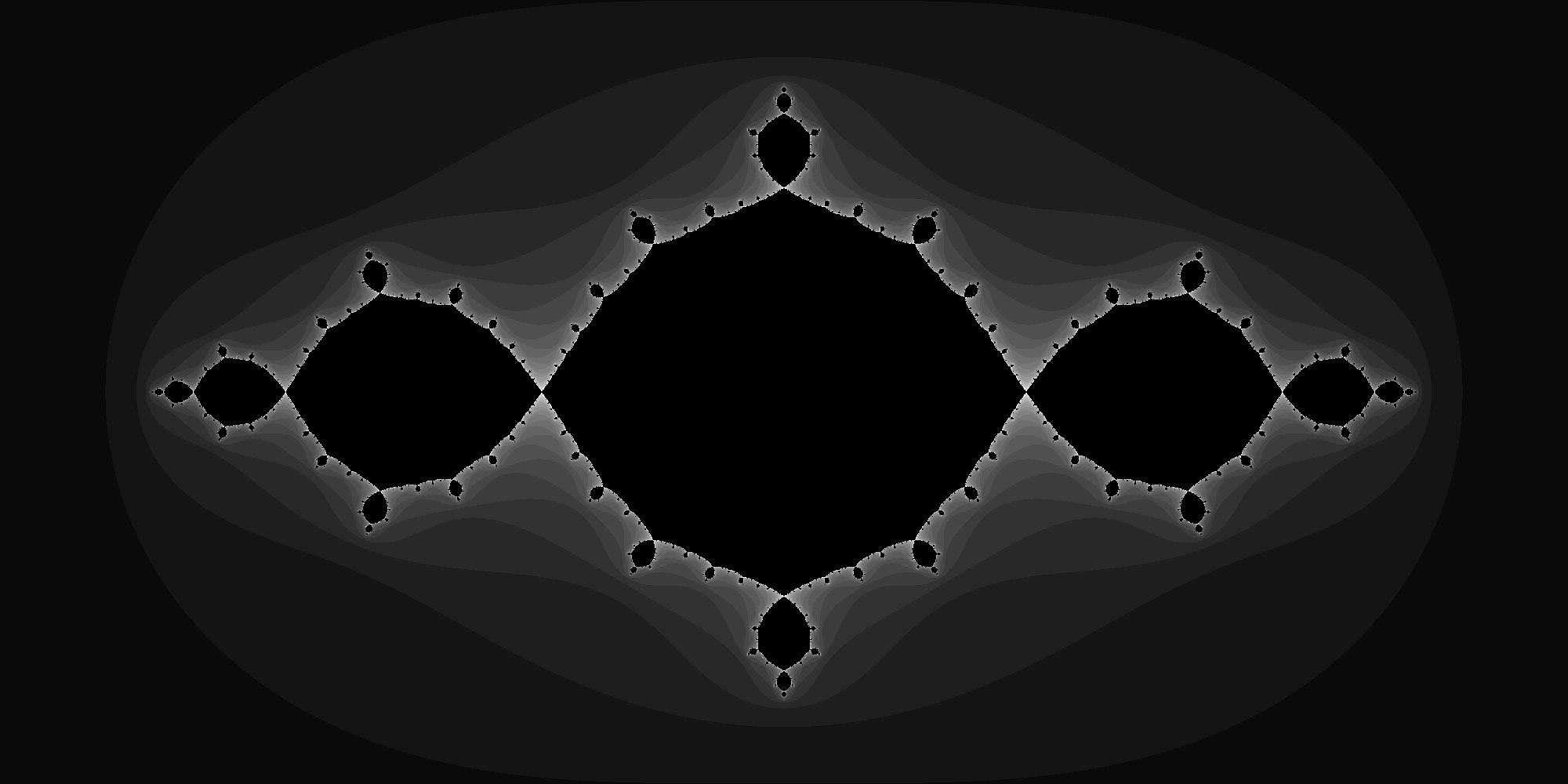
(If you’re wondering about that x -> 10x bit, it just scales the iteration count before we feed it to grayvalue. The |> is just a convenient operator for function composition (read: fewer parentheses), similar to, for example, F#. Oh, and numeric coeffients like 10 above imply multiplication).
That’s a good start, but the simple mapping of discrete iteration count to gray level leads to distinct “bands” in the final image. Ideally, we would like to have a continuously varying output of the boundedorbit function so that we could in turn have continuously changing color in the final image. We are not the first to encounter this problem, and there are published techniques for dealing with it (see this paper); we will use a common method called the normalized iteration count algorithm. Without going into details, this algorithm has the desirable property that it closely matches the values produced by the usual escape time method, but continuously. The formula is \[ n + \frac{\log\left(\log b\right) - \log\left( \log |z_{n}| \right)}{\log 2} \] where \(n\) is the iteration count, \(b\) is the bailout radius and \(z_{n}\) is the \(n\)-th iterate of the initial value.
Translating this formula into Julia code is a trivial exercise:
normalized_iterations(n, zn, bailout) = n + (log(log(bailout))-log(log(abs(zn))))/(log(2))Now we are equipped to produce a continuously colored version of the above image:
values = map(z -> boundedorbit(x -> x^2 - 1, z, 2, 500, normalized_iterations)
               |> x -> 10x
               |> grayvalue, linspace(-2-1im, 2+1im, 2000, 1000));
image = grayim(values)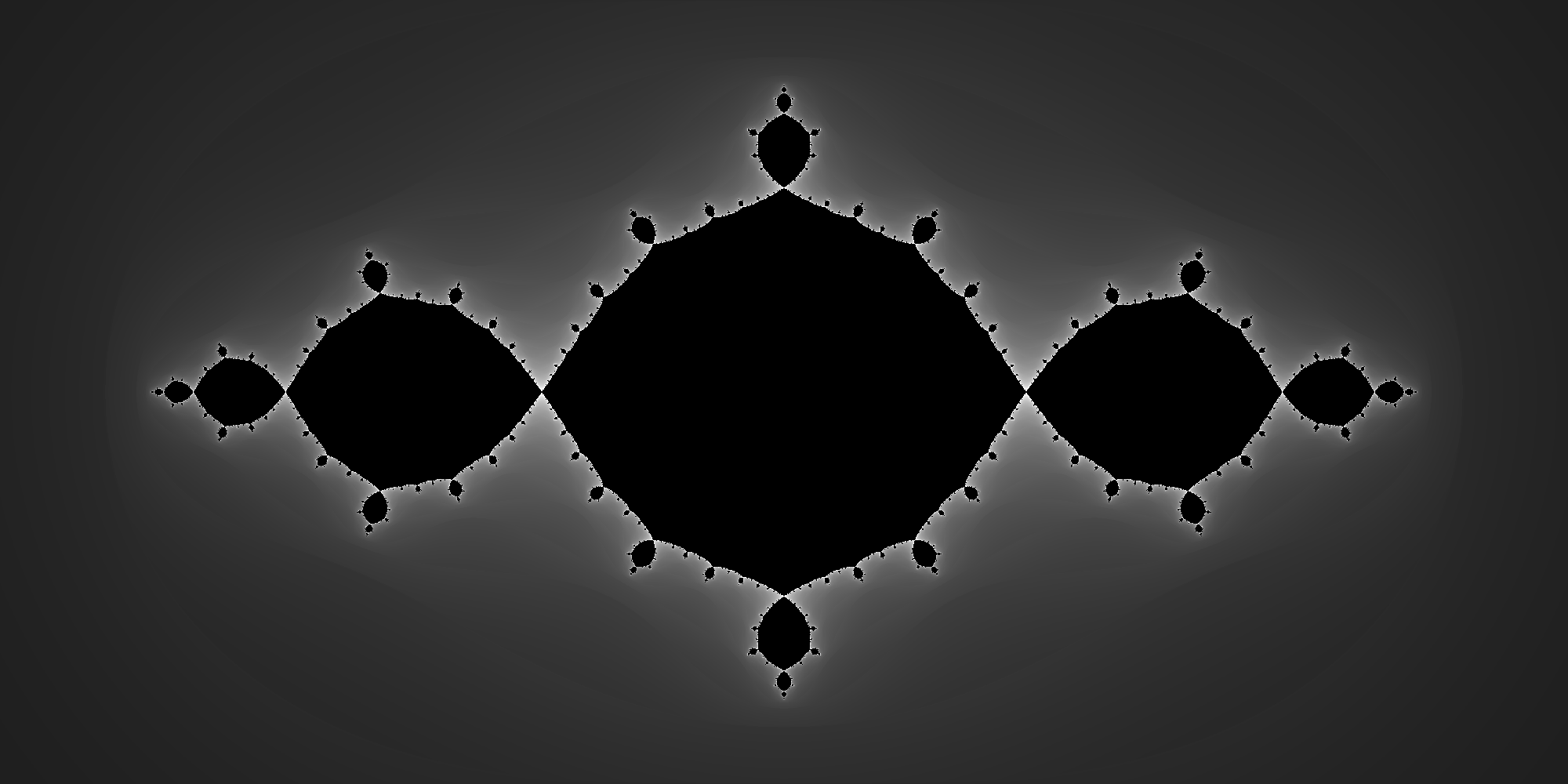
A little different initial seed value results in an altogether different and sublimely beautiful image:
values = map(z -> boundedorbit(x -> x^2 - (0.70176+0.3842im), z, 3, 200, normalized_iterations)
               |> x -> 3x
               |> grayvalue, linspace(-2-1im, 2+1im, 2000, 1000));
image = grayim(values)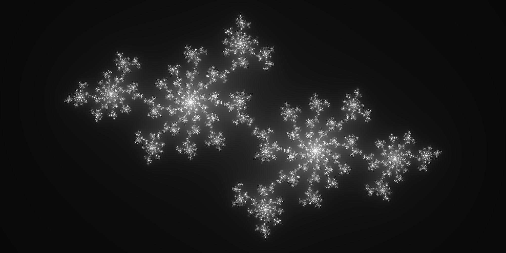
One more variation, and then we’ll move on.
values = map(z -> boundedorbit(z -> z^2 + 0.285+0.01im, z, 3, 500, normalized_iterations)
               |> grayvalue, linspace(-2-2im, 2+2im, 2000, 2000));
image = grayim(values)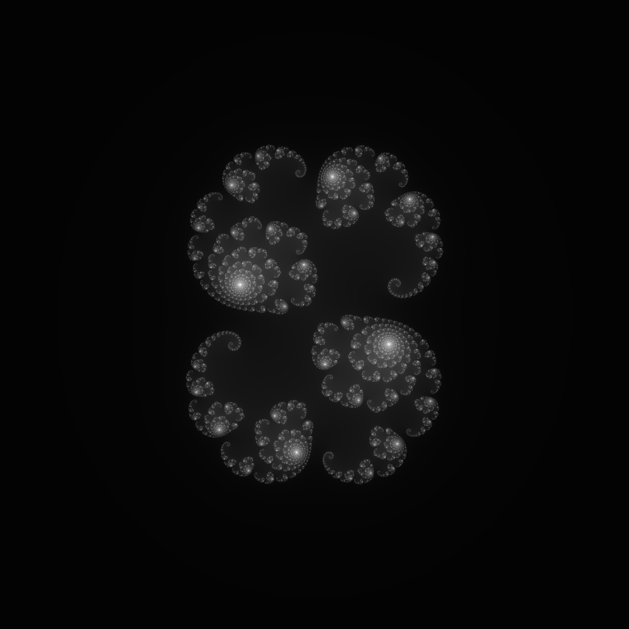
An interesting (and perhaps familiar!) thing happens when instead of varying the initial seed value, we always start with a seed of zero and instead vary the constant \(c\) in the function \(z^2 + c\):
values = map(z -> boundedorbit(x -> x^2 + z, 0, 2, 200, normalized_iterations)
               |> x -> 5x
               |> grayvalue, linspace(-2.5-1.25im, 1.0+1.25im, 3500, 2500));
image = grayim(values)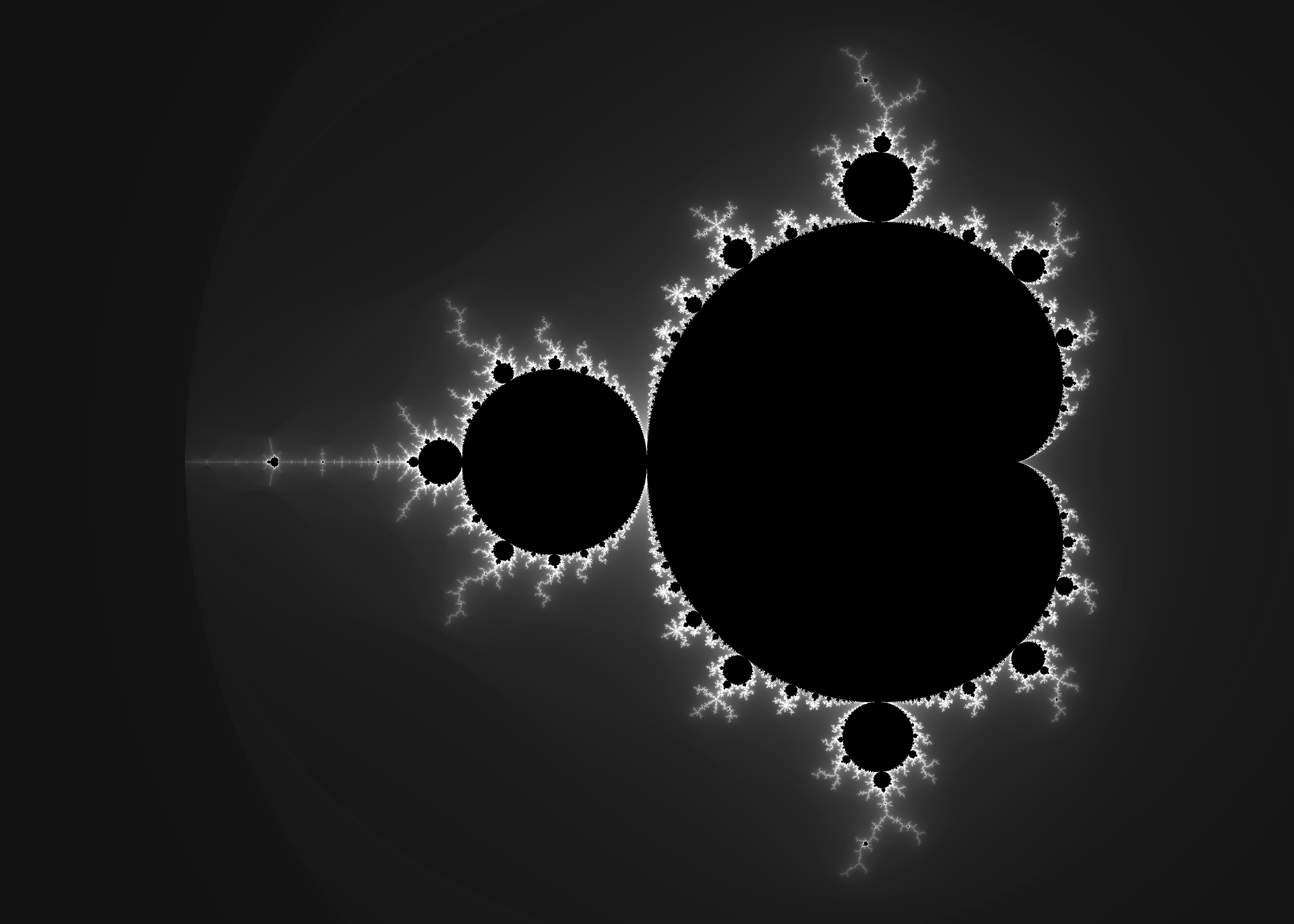
This is, of course, the famous Mandelbrot Set. Now, I find these grayscale images have a certain elegance, but what if we wanted to add a little color? After all, that’s the way you usually find these fractals rendered. As it happens, Julia’s package database includes a Color package that may be the most comprehensive library for working with colors and colorspaces that I’ve ever encountered. Our needs here will hardly scratch the surface. To begin with, let’s make a color monochrome variant of grayvalues by taking one color and scaling its saturation and value with the iteration count:
using Color

function colorvalue(n)
    HSV(225.0, 1.0-clamp(n/50.0, 0, 1.0), clamp(n/50.0, 0, 1.0))
end
HSV is a handy type from the Colors package; there are many more. Now let’s see how that looks:
colors = map(z -> boundedorbit(x -> x^2 + z, 0, 2, 100, normalized_iterations)
               |> colorvalue, linspace(-2.5-1.25im, 1.0+1.25im, 3500, 2500))
image = convert(Image{RGB}, Image(colors, spatialorder=["x","y"]))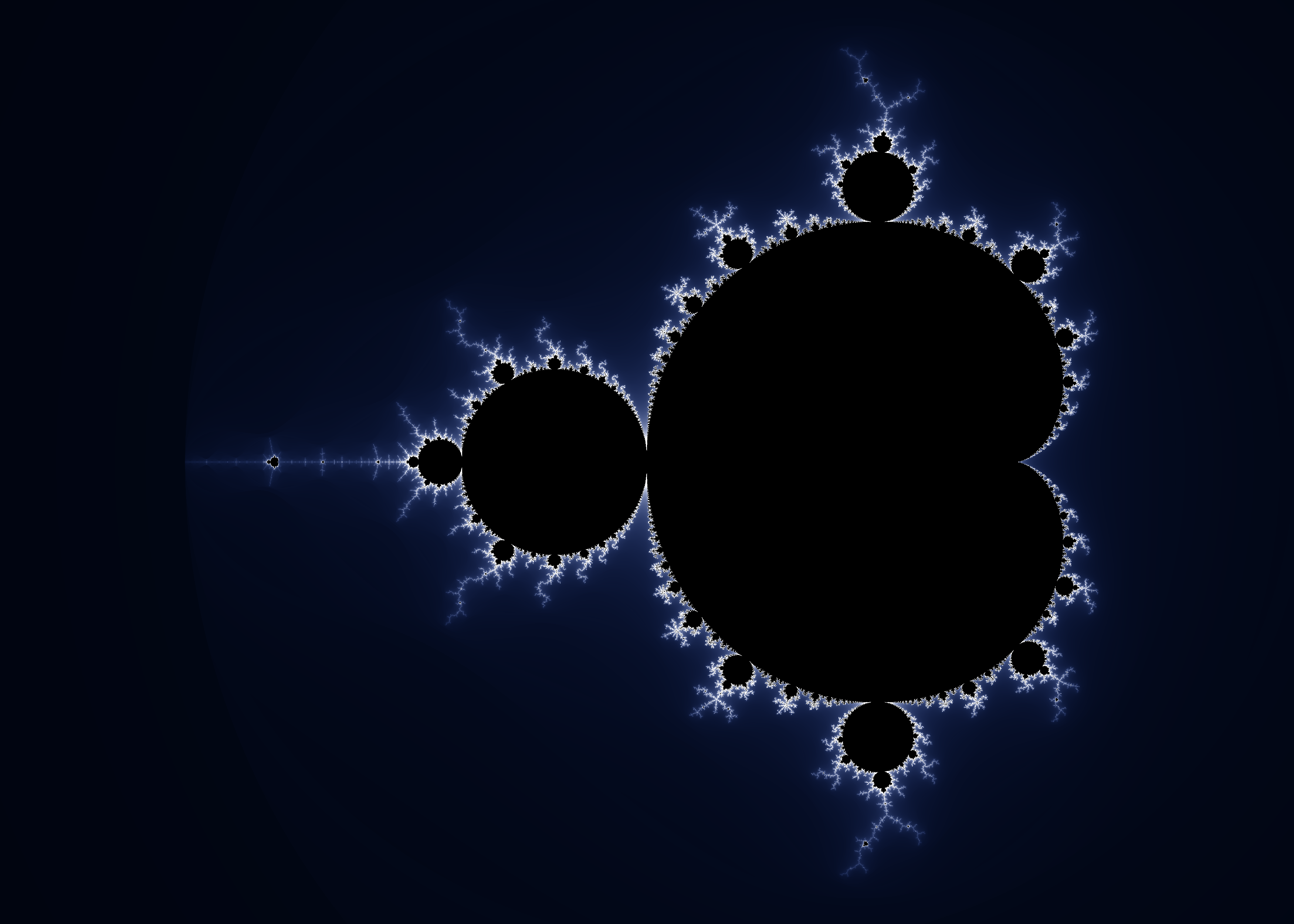
A pleasing result, but let’s try one more thing. The Color package provides a convenient means of creating arbitrary palettes or gradients, which in reality are just Array’s of color values. For example, here’s a 10-step color palette:
Now we’re going to want more than 12 discrete values for coloring our fractal; by increasing the number of steps we can get something like this:
Finally, we need a new function to map iterations into our color palette.
function interpolate_palette(palette, n)
    if n == -Inf
        RGB(0,0,0)
    else
        palette[iround(clamp(n,1,length(palette)))]
    end
end
Finally, we end up with this:
palette = diverging_palette(240.0, 80.0, 20000, mid=0.125)[1:10000];
colors = map(z -> boundedorbit(x -> x^2 + z, 0, 2, 300, normalized_iterations)
               |> n -> interpolate_palette(palette, sign(n)*n^2.2), linspace(-2.5-1.25im, 1.0+1.25im, 3500, 2500));
image = convert(Image{RGB}, Image(colors, spatialorder=["x","y"]))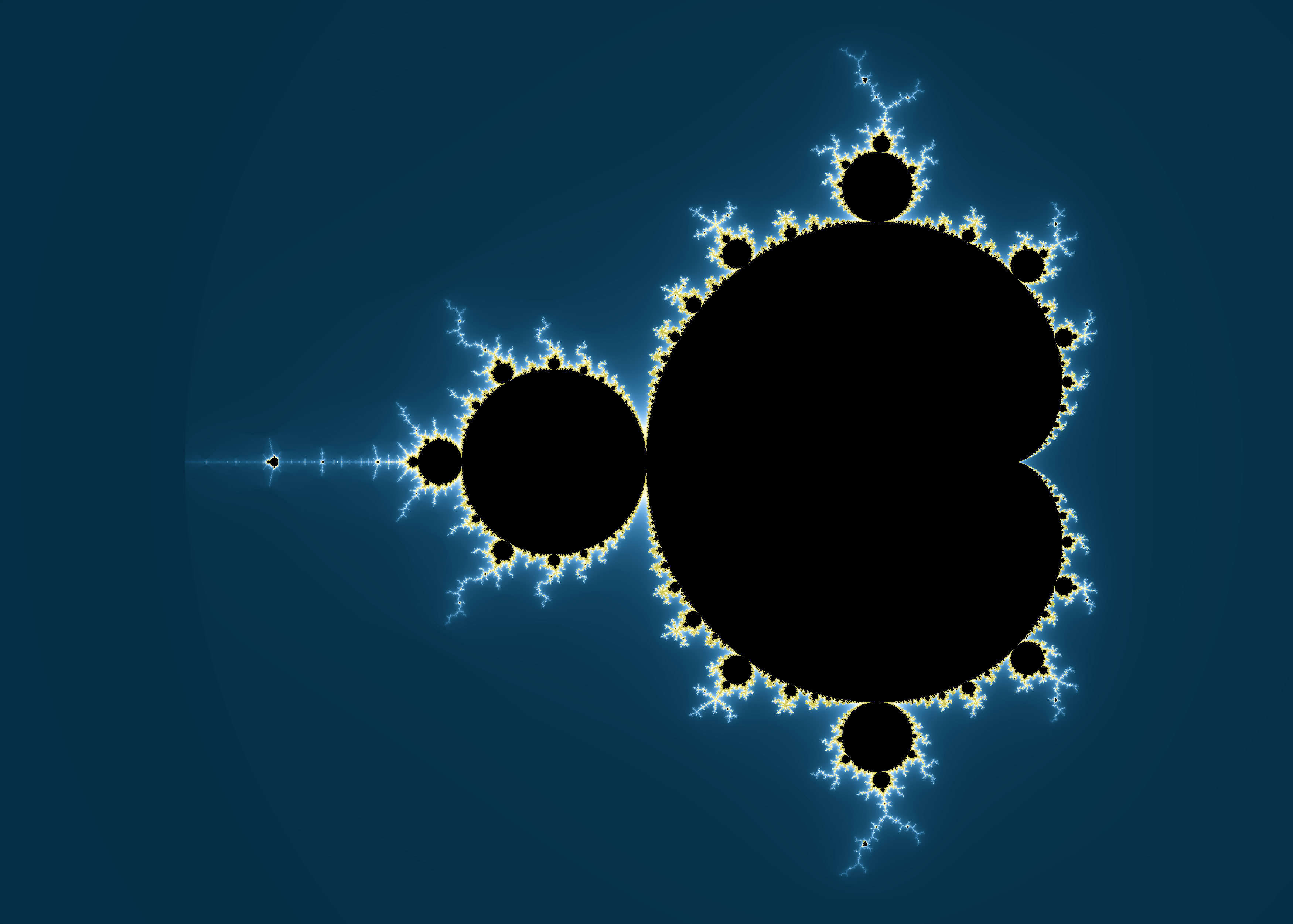
I’ve only scratched the surface of what you can do with Julia, let alone the beautiful mathematics behind the images. If you want to learn more about Julia, have a look at the execellent documentation, or try the learning resources. If you’re interested in the mathematics of fractals, this book is hard to beat.